Credit, funding, margin, and capital valuation adjustments for bilateral portfolios

Abstract

We apply to the concrete setup of a bank engaged into bilateral trade portfolios the XVA theoretical framework of (Albanese and Crépey2017), whereby so-called contra-liabilities and cost of capital are charged by the bank to its clients, on top of the fair valuation of counterparty risk, in order to account for the incompleteness of this risk. The transfer of the residual reserve credit capital from shareholders to creditors at bank default results in a unilateral CVA, consistent with the regulatory requirement that capital should not diminish as an effect of the sole deterioration of the bank credit spread. Our funding cost for variation margin (FVA) is defined asymmetrically since there is no benefit in holding excess capital in the future. Capital is fungible as a source of funding for variation margin, causing a material FVA reduction. We introduce a specialist initial margin lending scheme that drastically reduces the funding cost for initial margin (MVA). Our capital valuation adjustment (KVA) is defined as a risk premium, i.e. the cost of remunerating shareholder capital at risk at some hurdle rate.

Introduction

Albanese and Crépey (2017) developed an XVA theoretical framework based on a capital structure model acknowledging the impossibility for a bank to replicate jump-to-default related cash flows. Their approach results in a two-step XVA methodology.

First, the so-called contra-assets (CA) are valued as the expected counterparty default losses and funding expenditures. These expected costs can be represented as the sum between the valuation, dubbed CR, of counterparty risk to the bank as a whole (or “fair valuation” of counterparty risk), plus an add-on compensating bank shareholders for a wealth transfer to creditors, corresponding to the so-called contra-liabilities (CL), triggered by the impossibility for the bank to hedge its own jump-to-default exposure.

Second, a KVA risk premium is computed as the cost of a sustainable remuneration of the shareholder capital at risk earmarked to absorb the exceptional (beyond expected) losses due to the impossibility for the bank to replicate counterparty jump-to-default cash flows.

The all-inclusive XVA add-on appears as

$$ \text{CA} +\text{KVA}=\text{CR} +\text{CL}+\text{KVA}. $$

(1)

This formula is applied for every new deal or tentative deal, incrementally on a run-off basis in the portfolios with and without the new deal, in order to derive the so-called funds transfer price (FTP) of the deal. The corresponding pricing policy is interpreted as the cost for the bank of the possibility to run-off its portfolio, in line with shareholder interest, from any future time onward if wished. This “soft landing” option is key from a regulator point of view, as it guarantees that the bank should not be tempted to go into snowball or Ponzi kind of schemes where always more trades are entered for the sole purpose of funding previously entered ones.

In the present paper we apply this framework to the concrete setup of a bank engaged in bilateral trade portfolios. In this context, the discounted expectation of losses due to the default of counterparties or of the bank itself are respectively known as CVA (credit valuation adjustment) and DVA (debt valuation adjustment). Counterparty risk mitigants include the variation margin (VM), tracking the mark-to-market of client portfolios, and the initial margin (IM) set as a cushion against gap risk, which is the risk of slippage between the portfolio and its variation margin during liquidation periods. The cost of funding cash collateral for the variation margin is known as funding valuation adjustment (FVA), while the cost of funding segregated collateral posted as initial margin is the margin valuation adjustment (MVA). Contra-liability counterparts of the FVA and the MVA arise as the FDA (funding debt adjustment) and the MDA (margin debt adjustment). The contra-liability component of a unilateral CVA is dubbed CVA^CL.

The main contributions of this paper are the concrete equations of Proposition 4.1 for the corresponding CA=CVA+FVA+MVA and KVA metrics, the XVA algorithm and the numerical results on real datasets. The refined FVA in (29) captures the intertwining of the FVA and economic capital, which leads to a significantly lower FVA as a result of the fungibility of economic capital (on top of reserve capital) as a source of funding for variation margin. The alternative MVA formula (30) shows how a specialist initial margin lending scheme may drastically reduce the funding cost for initial margin (MVA).

Assumptions are emphasized in bold throughout the paper.

XVA conceptual framework

This section provides a brief recap of the XVA methodology that arises from Albanese and Crépey (2017).

We consider a bank made of four different floors. The intermediate floors (CVA and Treasury) are in charge of filtering out counterparty risk and its risky funding implications from the contracts with the clients of the bank. In the case of the Treasury there are two desks on the same floor (sharing the same bank account): the FVA desk, in charge of funding the VM, and the MVA desk, in charge of funding the IM. The upper floor is the management in charge of the KVA payments to the shareholders, i.e. of the dividend distribution policy of the bank. Thanks to the upper floors of the bank, the traders of the bottom (dubbed clean) floor can focus on the management of the market risk of their respective business lines, ignoring counterparty risk and its capital and funding implications.

CVA payments by clients flow into a a reserve credit (RC) account used by the CVA desk for coping with expected counterparty default losses. FVA and MVA payments flow into a reserve funding (RF) account used by the Treasury for coping with expected funding expenditures. KVA payments flow into a risk margin (RM) account from which they are gradually released by the bank management to shareholders as a remuneration for their capital at risk. We assume that all bank accounts are continuously reset to their theoretical target level. Therefore, the relations

$$ {}\left\{ \begin{array}{l} \!\text{RC}\,=\,\text{CVA}\text{ and }\text{RF}\,=\,\text{FVA}\!+\text{MVA},\text{ hence } \text{RC}+\text{RF}=\text{CVA}+\text{FVA}+\text{MVA}=\text{CA}\\ \!\text{RM}\,=\,\text{KVA} \end{array} \right. $$

(2)

hold at all times. In particular, much like with futures, the trading position of the bank (clean desks, CVA desk and Treasury altogether) is reset to zero at all times, but it generates a non-vanishing (unless perfectly hedged) trading loss-and-profit process L, or loss process for brevity. The KVA payments by the management of the bank come on top of the trading gains as an additional contribution to shareholder dividends, which corresponds to risk compensation.

In order to focus on counterparty risk and XVA analysis, we assume throughout the paper that the clean desks of the bank are perfectly hedged, i.e. their trading loss is zero. Hence, only the counterparty risk related cash flows remain and we can concentrate on the activity of the CVA floor, the Treasury and the management of the bank.

The default of the bank is modeled as a totally unpredictable time τ calibrated to the bank CDS spread, which we view as the most reliable and informative credit data regarding anticipations of markets participants about future recapitalization, government intervention, etc. Assuming instantaneous liquidations upon defaults, the time horizon of the model is $\bar {\tau }=\tau \wedge T,$ where T is the final maturity of the portfolio.

We assume that, at the bank default time τ , an exceptional (e.g. operational) loss occurs and wipes out any residual risk capital (shareholder capital at risk and risk margin) and reserve funding capital, whereas the residual credit capital is transferred to creditors, who need it for coping with counterparty defaults after the bank default (in which case, creditors must mark to market a loss on the derivative position of the bank; similarly, if the creditors unwind the position of a counterparty, they have to recognize a CVA discount.

We consider a pricing stochastic basis $(\Omega,\mathbb {G},\mathbb {Q}),$ with model filtration $\mathbb {G}=(\mathfrak {G}_{t})_{t\in \mathbb {R}_{+}}$ and probability measure $\mathbb {Q},$ such that all processes of interest are $\mathbb {G}$ adapted and all random times of interest are $\mathbb {G}$ stopping times. The corresponding expectation and conditional expectation are denoted by $\mathbb {E}$ and $\mathbb {E}_{t}$. All value and price processes are modeled as semimartingales in a càdlàg version.

We denote by r a $\mathbb {G}$ progressive OIS rate process, where OIS rate stands for overnight indexed swap rate, which is together the best market proxy for a risk-free rate and the reference rate for the remuneration of cash collateral. We write $\beta _{t}=e^{-\int _{0}^{t} r_{s} ds}$ for the corresponding risk-neutral discount factor. We denote by the survival indicator process of the bank. For any left-limited process Y, we denote by Δ _τ Y=Y _τ −Y _τ− the jump of Y at τ and by Y ^τ−=JY+(1−J)Y _τ− the process Y stopped before τ, so that

$$ dY_{t} = dY^{\tau-}_{t}+(- \Delta_{\tau} Y)\, dJ_{t},\, 0\le t\le \bar{\tau}. $$

(3)

We say that the process Y is stopped before τ if Y=Y ^τ−.

Valuation

We denote by $\mathcal {C},\mathcal {F}$ and $\mathcal {M}$ the cumulative streams of counterparty exposure cash flows and of VM and IM related risky funding cash flows. By risky funding cash flows we mean the funding cash flows other than risk-free accrual of the bank accounts and risk-free remuneration of the collateral. Cash flows are valued by their risk-free discounted $(\mathbb {G},\mathbb {Q})$ conditional expectation, which is assumed to exist for all the cash flows that appear in the paper. Risky funding is implemented in practice as the stochastic integral of predictable hedging ratios against funding assets. Under the above valuation assumption for cash flows, the value process of each of these assets is a martingale modulo risk-free accrual. Hence $\boldsymbol{\boldsymbol{\boldsymbol{\mathcal {F}}}}$ and $\boldsymbol{\boldsymbol{\boldsymbol{\mathcal {M}}}}$ are $(\mathbb {G},\mathbb {Q})$ martingales. Moreover the trading desks of the bank is supposed to be shareholder-centric, in the sense that traders only value the cash flows that affect the shareholders of the bank, i.e. the cash flows received by the bank prior its default or the transfer from shareholders to creditors of the residual value on their trading account at the bank default time τ .

Proposition 2.1

We have, for $0\leq t\leq \bar {\tau },$

The trading loss process L of the bank is a risk-neutral local martingale such that

$$ \begin{aligned} &\beta_{t} dL_{t}=d\left(\beta_{t} \text{CA}_{t}\right)+\beta_{t} \left(d \mathcal{C}^{\tau-}_{t} + d\mathcal{F}^{\tau-}_{t} + d\mathcal{M}^{\tau-}_{t}\right),\, 0\leq t\leq \bar{\tau}, \end{aligned} $$

(5)

starting from some initial value L ₀=z unknown but immaterial, as only the fluctuations of L matter in capital computations.

Proof

In (4) the CA equations express the valuation of the cash flows that affect each of the trading desks before bank default (CVA, FVA and MVA desks, as clean desks disappear from the picture under our perfect clean hedge assumption). Moreover, the terminal cash flow in the CVA equation corresponds to the freezing of the residual credit capital RC _τ−=CVA _τ− (cf. (2)), which is transferred from bank shareholders to creditors in case of default of the bank. This results in a CVA terminal condition CVA _T =0 on {T<τ} and Δ _τ CVA=0 on {τ<T}, as embedded in the CVA equation in (4). This comes in contrast with the terminal conditions $\text {FVA}_{\bar {\tau }}=\text {MVA}_{\bar {\tau }}=0,$ which hold by our assumption that the residual funding capital is used for absorbing the exceptional loss of the bank at time τ. In line with the respective definitions (see “Introduction” section), we have

$$\begin{aligned} &\text{CR}_{t}=\mathbb{E}_{t}\int_{t}^{\bar{\tau}} \beta_{t}^{-1}\beta_{s} \left(d\mathcal{C}_{s}+d\mathcal{F}_{s}+d\mathcal{M}_{s}\right),\, &\text{CL}_{t}=\text{CA}_{t}-\text{CR}_{t}, \end{aligned} $$

from which the expressions stated for CR and CL in (4) result by the martingale properties of $\mathcal {F}$ and $\mathcal {M}$ and the CA equations in (4).

Note that the CVA, FVA and MVA equations in (4) are equivalent to the above-mentioned terminal conditions, alongside with martingale conditions on the following processes on $[0,\bar {\tau } ]$, which correspond to the trading loss processes of the corresponding trading desks:

$$ \begin{aligned} &\beta_{t} d{L}^{cva}_{t} =d\left(\beta_{t}{\text{CVA}}^{\tau-}_{t}\right)+\beta_{t} d\mathcal{C}^{\tau-}_{t}\\ &\beta_{t} d{L}^{fva}_{t}= d(\beta_{t}{\text{FVA}}_{t}) +\beta_{t} d\mathcal{F}^{\tau-}_{t}\\ &\beta_{t} d{L}^{mva}_{t}= d(\beta_{t}{\text{MVA}}_{t}) +\beta_{t} d\mathcal{M}^{\tau-}_{t}, \end{aligned} $$

(6)

Under our perfect clean hedge assumption, these add-up to the trading loss L of the bank (the KVA payments by the management of the bank are not part of the trading losses but risk compensation to shareholders). This yields the Eq. (5) for L (noting that the CVA process is stopped before τ). □

We emphasize that Proposition 2.1 is derived from a pure valuation perspective. In most references in the literature, XVA equations are based on hedging arguments. The reason is that previous XVA works were not considering KVA yet. Under our approach, the KVA is the risk premium for the market incompleteness related to the impossibility for the bank of replicating counterparty default losses. For consistency, our KVA treatment requires a pure valuation (as opposed to hedging) treatment of contra-assets and contra-liabilities.

Note that the CVA formula in (4) is in fact a fixed-point equation, which remains to be shown well posed in a suitable space of processes. Even if not visible at that stage, this remark also applies to the FVA equation, as the risky funding cash flows $\mathcal {F}$ typically depend on the FVA itself (cf. e.g. (17), where CA includes an FVA term).

Pricing

In the setup of Albanese and Crépey (2017), valuation is not price, which entails an additional deduction in the form of the KVA risk premium devised by the management of the bank in order to compensate the shareholders for their capital at risk. In the absence of reliable information about it at the time horizon of XVA computations (which can be as long as decades), we assume that the historical probability measure $\mathbb {P}$ required for capital calculations coincides with the pricing measure $\mathbb {Q}$, the discrepancy between $\mathbb {P}$ and $\mathbb {Q}$ being left to model risk.

Since L fluctuates over time according to (5), economic capital EC=EC _t (L) needs to be dynamically earmarked by the bank in order to absorb exceptional losses (beyond the expected level of the losses already accounted for by reserve capital). As shown in Albanese and Crépey (2017, Sections 4.3, 6.5 and 8.1) the size of the risk margin (RM) account required for remunerating shareholder capital at risk (SCR) at a constant hurdle rate h throughout the life of the portfolio is

$$ \begin{aligned} \text{KVA}_{t} =h \mathbb{E}_{t} \int_{t}^{\bar{\tau}} e^{-\int_{t}^{s} (r_{u} +h) du} \text{EC}_{s}(L) ds,\,t\in[0,\bar{\tau}], \end{aligned} $$

(7)

where EC _s (L) is computed based on a

$$ \text{97.5\% expected shortfall (ES) of } \int_{s}^{s+1}\beta_{s}^{-1} \beta_{u} dL_{u} \text{ conditional on } \mathfrak{G}_{s}, $$

(8)

which we denote by ES _s (L).

The “ +h” in the discount factor in (7) reflects the fact that the risk margin RM=KVA (cf. (2)) is loss-absorbing, hence part of EC, so that shareholder capital at risk reduces to SCR = EC − KVA. As a further consequence of this loss-absorbing feature of the risk margin, an increase of economic capital above ES may be required in order to ensure the consistency condition KVA≤EC, i.e. EC−KVA=SCR≥0. This results in a fixed-point problem (7), where

$$ \begin{aligned} \text{EC}_{t}(L)=\max\left(\text{ES}_{t}(L),\text{KVA}_{t}\right),\, t\in[0,\bar{\tau}]. \end{aligned} $$

(9)

Remark 2.1

For KVA computations entailing capital projections over decades, an equilibrium view based on Pillar II economic capital (EC) is more attractive than the ever-changing Pillar I regulatory charges supposed to approximate it (see Pykhtin (2012)). However, Pillar I regulatory capital requirements could be incorporated into our approach, if desired, by replacing ES=ES _t (L) in (9) by its maximum with the regulatory capital pertaining to the portfolio.

Bilateral trading cash flows

In this paper, we assume that the bank is engaged in bilateral trading of a derivative portfolio split into several netting sets corresponding to counterparties indexed by i=1,…,n, with default times τ _i and survival indicators . The bank is also default prone, with default time τ and survival indicator .

We suppose that all these default times are positive and admit a finite intensity. In particular, defaults occur at any given $\mathbb {G}$ predictable stopping time with zero probability, so that such events can be ignored in all computations.

Exposures at defaults

Let $\text {MtM}^{i}_{t}$ be the mark-to-market of the i-th netting set, i.e. the trade additive risk-neutral conditional expectation of future discounted promised cash flows, ignoring counterparty risk and assuming risk-free funding. Let $\text {VM}^{i}_{t}$ denote the corresponding variation margin, counted positively when received by the bank. Hence,

$$ P^{i}_{t} = \text{MtM}^{i}_{t} - \text{VM}^{i}_{t} $$

(10)

is the net spot exposure of the bank to the i-th netting set. In addition to the variation margin $\text {VM}^{i}_{t}$ that flows between them, the bank and counterparty i post respective initial margins PIMⁱ and $\text {RIM}^{i}_{t}$ in some segregated accounts.

In practice, there is a positive liquidation period, usually a few days, between the default of a party and the liquidation of its portfolio. The gap risk of slippage of MtM$^{i}_{t}$ and of unpaid contractual cash flows during the liquidation period is the motivation for the initial margin.

A positive liquidation period is explicitly introduced in Armenti and Crépey (2017a, b) and Crépey and Song (2016) (see also Brigo and Pallavicini (2014)) and involves introducing the random variables

$$ \text{MtM}^{i}_{\tau_{i} + \delta{t}} + \delta \text{MtM}^{i}_{\tau_{i} + \delta{t}} - \text{VM}^{i}_{\tau_{i}}, $$

(11)

where δ t is the length of the liquidation period and $\delta \text {MtM}^{i}_{\tau _{i} + \delta {t}}$ is the accrued value of all cash flows owed by the counterparty to the bank during the liquidation period.

To simplify the notation in this paper, we take the limit as δ t→0 and approximate $\text {MtM}^{i}_{\tau _{i} + \delta {t}} + \delta \text {MtM}^{i}_{\tau _{i} + \delta {t}}$ with $\widehat {\text {MtM}}^{i}_{\tau _{i}}$, and therefore (11) by $Q^{i}_{\tau _{i}}=\widehat {\text {MtM}}_{\tau _{i}}^{i}- \text {VM}_{\tau _{i}}^{i}$, for a suitable $\mathbb {G}$ optional process $\widehat {\text {MtM}}^{i}$. A related issue is wrong-way risk, i.e. the risk of adverse dependence between the counterparty exposure and the credit risk of the parties. As illustrated in Crépey and Song (2016), this impact can also be captured in the modeling of the $Q^{i}_{\tau _{i}}$.

We denote by R and R _i the recovery rate of the bank and of counterparty i, for i=1,…,n.

Lemma 3.1

The exposure of the bank to the default of counterparty i=1,…,n at time τ _i ≤τ∧T is

$$ \begin{aligned} \left(1-R_{i}\right) \left(Q^{i}_{\tau_{i}} - \text{RIM}^{i}_{\tau_{i}}\right)^{+}. \end{aligned} $$

(12)

The exposure of counterparty i=1,…,n to the default of the bank at time τ≤τ _i ∧T is

$$\begin{aligned} (1-R) \left(Q^{i}_{\tau} - \text{PIM}^{i}_{\tau }\right)^{-}. \end{aligned} $$

(13)

Proof

By symmetry, it is enough to prove (12). Let C ⁱ=VMⁱ+RIMⁱ and

$$\epsilon_{i}=\left(Q^{i}_{\tau_{i}}-\text{RIM}^{i}_{\tau_{i}}\right)^{+}=\left(\widehat{\text{MtM}}^{i}_{\tau_{i}}- {C}^{i}_{\tau_{i}} \right)^{+}. $$

When counterparty i defaults, the bank receives from counterparty i

Also accounting for the unwinding of the clean hedge of netting set i at the time of liquidation of counterparty i, the loss of the bank in case of default of counterparty i appears as (assuming τ _i ≤τ)

□

As an immediate corollary to Lemma 3.1, denoting by δ _t a Dirac measure at time t:

Lemma 3.2

The cumulative cash flow stream $\mathcal {C}$of counterparty exposures satisfies, for $0\le t\le \bar {\tau },$

$$ \begin{aligned} d\mathcal{C}_{t}\!&=\! \sum\limits_{i}\! \left(1\,-\,R_{i}\right) \!\left(Q^{i}_{\tau_{i}} \!- \text{RIM}^{i}_{\tau_{i}}\right)^{+}\! \boldsymbol\delta_{\tau_{i}}\!(dt\!)\,-\,\!\sum\limits_{i}\! J^{i}_{\tau-} (1\,-\,R)\! \left(Q^{i}_{\tau}\! -\! \text{PIM}^{i}_{\tau }\right)^{-}\! \boldsymbol\delta_{\tau}\!(dt\!)\\ d\mathcal{C}^{\tau-}_{t}&= \sum\limits_{i} J_{\tau_{i}} (1-R_{i}) \left(Q^{i}_{\tau_{i}} - \text{RIM}^{i}_{\tau_{i}}\right)^{+} \boldsymbol\delta_{\tau_{i}}(dt) \\ \left(-\Delta_{\tau}\mathcal{C} \right)&=\sum\limits_{i} J^{i}_{\tau-}(1-R) \left(Q^{i}_{\tau} - \text{PIM}^{i}_{\tau }\right)^{-} \boldsymbol\delta_{\tau }(dt)\\ & \quad- \sum\limits_{i;\tau_{i}=\tau}(1-R_{i}) \left(Q^{i}_{\tau_{i}} - \text{RIM}^{i}_{\tau_{i}}\right)^{+} \boldsymbol\delta_{\tau_{i}}(dt). \end{aligned} $$

(14)

Margining and funding schemes

Variation margin typically consists of cash that is re-hypothecable, meaning that received variation margin can be reused for funding purposes, and is remunerated at OIS by the receiving party. Initial margin typically consists of liquid assets deposited in a segregated account, such as government bonds, which naturally pay coupons or otherwise accrue in value. The poster of initial margin receives no compensation, except for the natural accrual or coupons of its collateral.

The trading strategy of the bank needs funding for raising variation margin and initial margin that need to be posted as collateral. As happens in practice in the current regulatory environment, the clean hedge of the derivative portfolio of the bank is assumed to be with other financial institutions and attracts variation margin at zero threshold (i.e. is fully collateralized), so that the variation margin posted by the bank on its hedge is constantly equal to $\sum _{i}J^{i} \text {MtM}^{i}$. Hence, the bank posts $\sum _{i}J^{i} \text {MtM}^{i}$ as VM on the hedge and receives $\sum _{i}J^{i} \text {VM}^{i}$ as VM on client trades, which nets to

$$\sum\limits_{i} J^{i}_{t}\text{MtM}^{i}_{t}-\sum\limits_{i }J^{i}_{t}\text{VM}^{i}_{t} = \sum\limits_{i} J^{i}_{t} P^{i}_{t}. $$

Moreover, the bank can use reserve capital as variation margin. Note that the marginal cost of capital for using capital as a funding source for variation margin is nil, because when one posts cash against variation margin, the valuation of the collateralized hedge is reset to zero and the total capital amount does not change. If, instead, the bank were to post capital as initial margin, then the bank would record a “margin receivable” entry on its balance sheet, which however cannot contribute to capital since this asset is too illiquid and impossible to unwind without unwinding all underlying derivatives. Hence, capital can only be used as VM, while it seems that IM must be borrowed entirely.

Under our continuous reset assumption (2), the amount (RC+RF) of reserve capital that can be used as VM coincides at all times with the theoretical CA value. The cash held by the bank, whether borrowed or received as variation margin, is deemed fungible across netting sets in a unique funding set. In conclusion,

$$ \begin{aligned} & (\text{VM funding needs})_{t} \,=\,\left(\sum\limits_{i} J^{i}_{t} P^{i}_{t} -\text{CA}_{t}\right)^{+},\, (\text{IM funding needs})_{t}\!=\sum\limits_{i} J^{i}_{t}\, \text{PIM}^{i}_{t}. \end{aligned} $$

(15)

We assume that the bank can invest at the OIS rate r _t and obtain unsecured funding at rate ( r _t + λ _t ) for funding VM and ( $r_{t}+\bar {\lambda }_{t}$ ) for funding IM, via two bonds of different seniorities issued by the bank, with respective recoveries R and $\bar {R}$. Given our standing valuation setup, it must hold that

$$ \begin{aligned} \lambda=(1-R)\gamma,\,\bar{\lambda}=(1-\bar{R})\gamma, \end{aligned} $$

(16)

where γ is the risk-neutral default intensity process of the bank.

We denote by d μ _t =γ _t dt+dJ _t the compensated jump-to-default martingale of the bank.

Lemma 3.3

The cumulative cash flow streams $\mathcal {F}$ and $\mathcal {M}$ of VM and IM related risky funding cash flows satisfy, for $0\le t\le \bar {\tau },$

$$ \begin{aligned} d\mathcal{F}_{t}&= (1-R)\left(\sum\limits_{i} J^{i}_{t-} P^{i}_{t-} -\text{CA}_{t-}\right)^{+} d\mu_{t}, d\mathcal{M}_{t}= \left(1-\bar{R}\right)\left(\sum\limits_{i} J^{i}_{t-} \text{PIM}^{i}_{t-}\right) d\mu_{t}\\ d\mathcal{F}^{\tau-}_{t}&= \left(\sum\limits_{i} J^{i}_{t} P^{i}_{t} -\text{CA}_{t}\right)^{+} {\lambda}_{t} dt,\, d\mathcal{M}^{\tau-}_{t}= \left(\sum\limits_{i} J^{i}_{t} \text{PIM}^{i}_{t}\right) \bar{\lambda}_{t} dt\\ \left(-\Delta_{\tau} \mathcal{F} \right)&= (1-R)\left(\sum\limits_{i} J^{i}_{\tau-} P^{i}_{\tau-}-\text{CA}_{\tau-}\right)^{+},\,\left(-\Delta_{\tau} \mathcal{M}\right) =\left(1-\bar{R}\right)\left(\sum\limits_{i} J^{i}_{\tau-} \text{PIM}^{i}_{\tau-}\right). \end{aligned} $$

(17)

Proof

In view of the above description, we have

$$\begin{aligned} & d\mathcal{F}^{\tau-}_{t}= (\text{VM funding needs})_{t} {\lambda}_{t} dt,\, d\mathcal{M}^{\tau-}_{t}= (\text{IM funding needs})_{t} \bar{\lambda}_{t} dt\\ &\!\left(\,-\,\Delta_{\tau} \mathcal{F}\right)\,=\, (1\,-\,R)(\text{VM funding needs})_{\tau-},\!\, \left(\,-\,\Delta_{\tau} \mathcal{M} \right)\,=\,\left(\!1\,-\,\bar{R}\right)\!(\text{IM funding needs})_{\tau-}, \end{aligned} $$

i.e.

$$\begin{aligned} &d\mathcal{F}_{t}=(\text{VM funding needs})_{t-}\left({\lambda}_{t} dt + (1-R) dJ_{t}\right)\\ &d\mathcal{M}_{t}=(\text{IM funding needs})_{t-}\left(\bar{\lambda}_{t} dt + (1-\bar{R}) dJ_{t}\right). \end{aligned} $$

Hence, given (16),

$$\begin{aligned} & d\mathcal{F}_{t}\,=\, (1\,-\,R)(\text{VM funding needs})_{t-} d\mu_{t},\, d\mathcal{M}_{t}\,=\, \left(\!1\,-\,\bar{R}\right)\!\left(\text{IM funding needs}\right)_{t-} d\mu_{t}. \end{aligned} $$

In view of (15), this yields (17). □

Bilateral trading XVA formulas

We work under the technical assumption that each of the martingales

This holds, in particular, when $\mathbb {G}$ is modeled as the progressive enlargement of a reference filtration $\mathbb {F}$ by the bank default time τ, in a basic immersion setup where $(\mathbb {F},\mathbb {Q})$ martingales are $(\mathbb {G},\mathbb {Q})$ martingales without jump at time τ (see the comments before Section 3 in Duffie et al. (1996) or in Collin-Dufresne et al. (2004, page 1379) and see the comments following (3.22) and (H.3) or the remarks following Proposition 6.1 in Bielecki and Rutkowski (2001)). The more general case, where immersion hypothesis is violated and the technical condition (18) does not hold, can also be considered, by dealing explicitly with the underlying enlargement of filtration issue. This is done in Albanese and Crépey (2017).

Proposition 4.1 yields a complete specification of all XVA metrics and of the loss process L required as input data in the KVA computations, in the case of a bank engaged in bilateral trade portfolios. It identifies the FTP (all-inclusive XVA add-on to the entry price) of a new trade as its incremental (CVA+FVA+MVA+KVA), the difference with the complete market formula (FTDCVA−FTDDVA) (cf. “Connection with the Duffie and Huang (1996) formula” section) being explained by the CL wealth transfer and the KVA risk premium, which are triggered by the impossibility for the bank to replicate jump-to-default exposures.

We denote by:

• $\mathcal {L}_{p},p\geq 1,$ the space of progressively measurable processes X over $[0,\bar {\tau }]$ such that $\mathbb {E} \left [\int _{0}^{\bar {\tau }} |X_{t}|^{p} dt\right ]< +\infty,$

• $\mathcal {S}_{2},$ the space of adapted càdlàg processes Y over $[0,\bar {\tau }]$ such that $\mathbb {E} \left [\sup _{t \in [0, \bar {\tau }]} Y_{t}^{2}\right ] < \infty$.

All our XVA processes are sought for in $\mathcal {S}_{2}$. In particular, we assume that the CVA equation in (4) has at most one solution in $\mathcal {S}_{2},$ as can be established in the invariance bank default time framework of Albanese and Crépey (2017).

Proposition 4.1

Assuming that r is bounded from below, that the CVA and MVA processes in (19) are in $\mathcal {S}_{2}$, and that the processes r,λ, and $\lambda \left (\sum _{i}J^{i} P^{i} -{CVA} -{MVA}\right)^{+}$ are in $\mathcal {L}_{2}$:

• (i) Contra-assets are given as

  $$ \begin{aligned} &{}\text{CA}_{t}\,=\,\underbrace{\mathbb{E}_{t}\!\!\! \sum\limits_{\!\!\{i;\,t<\tau_{i} <T\}}\beta_{t}^{-1}\beta_{\tau_{i}} (1-R_{i}) \left(Q^{i}_{\tau_{i}} - \text{RIM}^{i}_{\tau_{i}}\right)^{+}}_{{\mathrm{{CVA}}_{t}}}\!+\underbrace{\mathbb{E}_{t}\int_{t}^{\bar{\tau}} \beta_{t}^{-1} \beta_{s} \bar{\lambda}_{s} \sum_{i} J^{i}_{s} \text{PIM}^{i}_{s} ds }_{{ \text{MVA}_{t}}}\\ &\ \ +\underbrace{\mathbb{E}_{t}\int_{t}^{\bar{\tau}} \beta_{t}^{-1} \beta_{s} \lambda_{s} \left(\sum_{i} J^{i}_{s} P^{i}_{s} - \text{CVA}_{s}-\text{MVA}_{s}-\text{FVA}_{s} \right)^{+} ds }_{{ \text{FVA}_{t}}},\, 0\le t\le \bar{\tau}, \end{aligned} $$

  (19)

  where FVA is the unique solution in $\mathcal {S}_{2}$ to the backward SDE (BSDE) defined by the last line.

• (ii) Contra-liabilities are given as

  

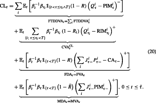
• (iii) The value of counterparty risk to the bank as a whole is given by

  

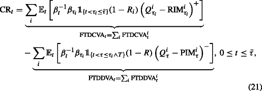
  i.e. we have

  $$ \begin{aligned} &\underbrace{\text{CVA}+\text{FVA}+\text{MVA}}_{\text{CA}} =\\ &\underbrace{\mathrm{{FTDCVA}}-\mathrm{{FTDDVA}}}_{\text{CR}}+ \underbrace{\mathrm{{FTDDVA}}+\text{CVA}^{\text{CL}} +\text{FDA} +\text{MDA}}_{\text{CL}}, \end{aligned} $$

  (22)

  where the different terms are detailed in (19), (20), and (21).

• (iv) The bank trading loss process L satisfies the following forward SDE on $[0,\bar {\tau }]$:

  $$ \begin{aligned} L_{0}&=z \text{ (the accrued trading loss of the bank at time {0}) and, for } t\in (0,\bar{\tau}],\\ dL_{t} &=d \text{CA}_{t} + \sum_{i} J_{\tau_{i}}(1-R_{i}) \left(Q^{i}_{\tau_{i}} - \text{RIM}^{i}_{\tau_{i}}\right)^{+} \boldsymbol{\delta}_{\tau_{i}}(dt)\\& \quad + \left(\lambda_{t} \left(\sum_{i} J^{i}_{t} P^{i}_{t} -\text{CA}_{t}\right)^{+} +\bar{\lambda}_{t} \sum_{i} J^{i}_{t} \text{PIM}^{i}_{t} -r_{t}\text{CA}_{t} \right) dt. \end{aligned} $$

  (23)

• (v) Assuming the ensuing ES=ES _t (L) process (8) in $\mathcal {L}_{2}$, KVA is the unique solution in $\mathcal {S}_{2}$ to the following BSDE:

  $$ \begin{aligned} \text{KVA}_{t} = h \mathbb{E}_{t} \int_{t}^{\bar{\tau}} e^{-\int_{t}^{s} \left(r_{u} +h\right) du} \max\left(\text{ES}_{s}(L),\text{KVA}_{s}\right) ds,\,t\in[0,\bar{\tau}]. \end{aligned} $$

  (24)

• (vi) The all-inclusive XVA add-on to the entry price for a new deal, which we call funds transfer price (FTP), appears as

  $$ \begin{aligned} \text{FTP}&= \underbrace{\Delta\text{CVA} +\Delta\text{FVA} +\Delta\text{MVA}}_{\mathrm{\Delta\text{CA}}} +\underbrace{\Delta\text{KVA}}_{\text{Risk~premium}}\\ &=\underbrace{\Delta\mathrm{{FTDCVA}}-\Delta\mathrm{{FTDDVA}}}_{\Delta\text{CR}}\\ &\quad + \underbrace{\Delta\mathrm{{FTDDVA}}+\Delta\text{CVA}^{\text{CL}} +\Delta\text{FDA} +\Delta\text{MDA}}_{\Delta\text{CL}} +\underbrace{\Delta\text{KVA}}_{\text{Risk~premium}}, \end{aligned} $$

  (25)

  computed on an incremental run-off basis, where all the underlying XVA metrics as well as the processes L to be used as input data in the economic capital and KVA computations are defined as in parts (i) through (v) relative to the portfolios with and without the new deal.

Proof

• (i) Denoting by UCVA (for unilateral CVA) the expression stated in (19) for the CVA, we have, on {t≤τ}:

  

  where the technical assumption (18) was used in the next-to-last equality. As a consequence,

  

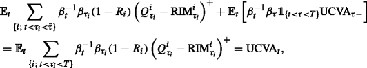
  by definition of UCVA. In view of (14), this means that the UCVA process satisfies the CVA equation in (4). Hence CVA = UCVA, by assumed uniqueness of an $\mathcal {S}_{2}$ solution to this equation.

  The MVA expression and FVA equation in (19) follow from the related equations in (4) and Lemma 3.3. In order to prove (i), it only remains to show that the FVA BSDE (last line in (19)) is well posed in $\mathcal {S}_{2}$. Let $X_{t}=\sum _{i}J^{i}_{t} P^{i}_{t} -\text {CVA}_{t} -\text {MVA}_{t}$. In terms of the coefficient

  $$\begin{aligned} f_{t} (y) =\lambda_{t} \left(X_{t} - y\right)^{+} - r_{t} y,\, y\in\mathbb{R}, \end{aligned} $$

  (26)

  the FVA BSDE is rewritten as

  $$ \begin{aligned} \text{FVA}_{t}=\mathbb{E}_{t} \int_{t}^{\bar{\tau}} f_{s} (\text{FVA}_{s}) ds,\, 0\le t\le \bar{\tau}. \end{aligned} $$

  (27)

  For any real $y,y'\in \mathbb {R}$ and $t\in [0,\bar {\tau }],$ we have

  $${}\begin{aligned} \left(f_{t}(y) - f_{t}(y')\right) (y-y')&=- r_{t} (y-y')^2+\lambda_{t} (y-y')\left(\left(X_{t} - y\right)^{+} -\left(X_{t} - y'\right)^{+}\right)\\ &\quad\leq - r_{t} (y-y')^{2} \leq C (y-y')^{2}, \end{aligned} $$

  for some constant C (having assumed r bounded from below and recalling λ≥0). Hence the BSDE coefficient f satisfies the so-called monotonicity condition. Moreover, for $|y|\leq \bar {y}$, we have:

  $$\begin{aligned} \left|f_{\cdot}(y)-f_{\cdot}(0)\right|&=\left|\lambda \left(X - y\right)^{+} - r y - \lambda X^{+} \right|\leq (\lambda+ | r |) \bar{y}. \end{aligned} $$

  Hence, assuming that r,λ and $\lambda \big (\sum _{i}J^{i} P^{i} -\text {CVA} -\text {MVA} \big)^{+}=\lambda X^{+}$ are in $\mathcal {L}_{2},$ the following integrability conditions hold:

  $$\begin{aligned} \sup_{|y|\leq \bar{y}}|f_{\cdot}(y)-f_{\cdot}(0)|\in {\mathcal{L}_{1}},\text{ for any } \bar{y}>0, \quad\text{and}\quad f_{\cdot}(0)\in {\mathcal{L}_{2}}. \end{aligned} $$

  Therefore, by application of the general filtration BSDE results of Kruse and Popier (2016, Sect. 5) the FVA BSDE (27) is well posed in $\mathcal {S}_{2}$.

• (ii) Follows from the CL equation in (4) and Lemmas 3.2– 3.3.

• (iii) The CR equation in (4) and Lemma 3.2 yield (21), after which (22) follows from (19), (20) and (21).

• (iv) Follows from (5) and Lemmas 3.2 – 3.3.

• (v) In view of (7) and (9), the KVA process satisfies the BSDE (24). This is a monotonic coefficient BSDE, which can be shown to be well posed in $\mathcal {S}_{2}$ much like the FVA BSDE in part (i) of the proof (see also Albanese and Crépey (2017, Section 6.3)).

• (vi) follows from (i) through (iv) by application of the generic formula (1), applied on an incremental run-off basis for every new trade as recalled after (1).

□

The regulator says quite explicitly that the bank capital (reserve capital in particular) cannot be seen increasing as a consequence of the sole deterioration of the bank credit, all else being equal (see Albanese and Andersen (2014, Section 3.1)). In particular, regulators decided that the CVA should be computed unilaterally, as in (19), by contrast with the first-to-default CVA (FTDCVA) in (21). As seen in the above, a unilateral CVA follows naturally from accounting for the wealth transfer corresponding to the transfer of the residual reserve credit from shareholders to creditors upon default of the bank.

In Proposition 4.1, the FVA appears as the solution to a BSDE through which it depends on all the CA components, including the FVA itself. This might seem in contradiction with our linear valuation rule for cash flows or with the additive appearance of the abstract FVA formula (4). The reconciliation between the two comes from the fact that the FVA is together value, by definition, and part RF=FVA of the amount in the reserve funding account, by (2). As RC+RF=CA is a deduction to the VM funding needs (cf. (2) and (15)), it follows that $\mathcal {F}$ in (17) depends on the FVA.

Connection with the Duffie and Huang (1996) formula

The formula (21) for the fair valuation CR of counterparty risk (valuation from the point of view of the bank as a whole) is derived inDuffie and Huang (1996) in the limit case of a perfect market (complete counterparty risk market without trading restrictions). Proposition 4.1 (iii) extends the validity of this fair valuation formula to our incomplete market setup.

Formula (21) is symmetrical, i.e. consistent with the law of one price, in the sense that each term (FTDCVAⁱ−FTDDVAⁱ) in (21) corresponds to the negative of the analogous quantity considered from the point of view of counterparty i. It only involves the first-to-default CVAs and DVAs, where the counterparty default losses are only considered until the first occurrence of a default of the bank or its counterparty in the deal. This is consistent with the fact, first pointed out in Duffie and Huang (1996) and later emphasized in Bielecki and Rutkowski (2002) and Brigo and Capponi (2008), that later cash flows will not be paid.

Since the presence of collateral has a direct reducing impact on FTDCVA/DVA, this formula may give the impression that collateralization achieves a reduction in counterparty risk at no cost to either the bank or the clients. However, in our incomplete market setup, the value CR of counterparty risk from the point of view of the bank as a whole ignores the misalignement of interest between the shareholders and the creditors of a bank. Propositions 4.1 (i) and (ii) give explicit decompositions of the shareholder valuation CA of counterparty risk and of the wealth transfer CL triggered from the shareholders to the creditors by the impossibility for the bank to hedge its own jump-to-default exposure (see Albanese and Crépey (2017, Sections 2.1 and 3.4)). Accounting for the further impossibility for the bank to replicate counterparty default losses, not only these contra-liabilities (CL), but also cost of capital (KVA), are material to shareholders and need to be reflected in entry prices on top of CR (cf. (1)).

Using economic capital as variation margin

In this section, we account for the FVA reduction provided by the possibility for a bank to post economic capital, on top of reserve capital RC+RF=CA already included in the above, as variation margin. Note that, in practice, uninvested capital of the bank can also be used for that purpose. But, since the amount of uninvested capital is unknown and could as well be zero in the future, capital is conservatively taken in FVA computations as CA+EC.

The quantity EC=EC _t (L) corresponds to the amount of economic capital required to cope with the loss process L (cf. (8)–(9)). Accounting for the use of EC as VM, the VM funding needs are reduced from $\left (\sum _{i} J^{i} P^{i} -\text {CA}\right)^{+}$ to $\left (\sum _{i} J^{i} P^{i} -{\text {EC}} (L)-\text {CA}\right)^{+}$ in (15). Lemma 3.3 is still valid provided one replaces $\left (\sum _{i} J^{i} P^{i} -\text {CA}\right)^{+}$ with $\left (\sum _{i} J^{i} P^{i} -{\text {EC}} (L)-\text {CA}\right)^{+}$ in (17).

As a consequence, instead of an exogenous CA value process as in (19) feeding the dynamics (23) for L, we obtain the following FBSDE system, made of a forward SDE for L coupled with a backward SDE for the FVA:

$$\begin{array}{@{}rcl@{}} L_{0}&=&z~\text{and, for } t\in (0,\bar{\tau}], \\ dL_{t} &=& {d \text{CA}_{t}}+ \sum_{i} J_{\tau_{i}}(1-R_{i}) \left(Q^{i}_{\tau_{i}} - \text{RIM}^{i}_{\tau_{i}}\right)^{+} \boldsymbol\delta_{\tau_{i}}(dt)\\ && + \left(\lambda_{t} \left(\sum_{i} J^{i}_{t} P^{i}_{t}-{\text{EC}}_{t}(L) -\text{CA}_{t}\right)^{+} +\bar{\lambda}_{t} \sum_{i} J^{i}_{t} \text{PIM}^{i}_{t} -r_{t}\text{CA}_{t} \right) dt, \end{array} $$

(28)

where

$$ \begin{aligned} \text{{FVA}}_{t}&=\mathbb{E}_{t}\int_{t}^{\bar{\tau}} \beta_{t}^{-1} \beta_{s} \lambda_{s} \left(\sum_{i} J^{i}_{s} P^{i}_{s} -{\text{EC}}_{s}(L)\right.\\ &\quad\left.-{\text{CVA}_{s}}-{\text{MVA}_{s}}-{\text{FVA}_{s}} {\vphantom{\sum_{i} J^{i}_{s} P^{i}_{s}}}\right)^{+} ds,\, 0\le t\le \bar{\tau} \end{aligned} $$

(29)

(whereas CVA and MVA are as in (19) and CA=CVA+FVA+MVA as usual).

Proceeding as in Crépey et al. (2017), one could show that, accounting for the use of economic capital as variation margin, Proposition 4.1 is still valid, provided one replaces $\left (\sum _{i} J^{i} P^{i} -\text {CA}\right)^{+}$ with $\left (\sum _{i} J^{i} P^{i} -{\text {EC}} (L)-\text {CA}\right)^{+}$ in all formulas.

Specialist lending of initial margin

If IM is unsecurely funded by the bank, then $\bar {\lambda }=\lambda$ in (19). However, instead of an unsecured IM funding scheme, one can consider a more efficient scheme where initial margin is funded through a specialist lender that lends only IM and, in case of default of the bank, receives back the portion of IM unused to cover losses.

Hence, the exposure of the specialist lender to the default of the bank is $(1-R) \sum _{i }J^{i}_{\tau } \left (\left (Q^{i}_{\tau }\right)^{-} \wedge \text {PIM}^{i}_{\tau }\right)$. Recalling the risk-neutral valuation condition λ=(1−R)γ in (16), where γ is the risk-neutral default intensity of the bank, the ensuing specialist lender MVA^sl is given as:

$$\begin{aligned} \text{{MVA}}^{sl}_{t}=\mathbb{E}_{t}\int_{t}^{\bar{\tau}} \beta_{t}^{-1} \beta_{s} {\lambda_{s}}\sum_{i} J^{i}_{s} \left(\left(Q^{i}_{s}\right)^{-} \wedge \text{PIM}^{i}_{s}\right) ds \end{aligned} $$

(30)

(assuming here for simplicity $\mathbb {G}$ predictable processes Q ⁱ and PIMⁱ). By identification with the general form $\bar {\lambda }_{t} \sum _{i }J^{i}_{t} \text {PIM}^{i}_{t}$ of instantaneous IM costs in this paper (cf. the generic MVA formula in (19)), this specialist lending scheme corresponds to

$$\bar{\lambda}_{t}=\frac{\sum_{i }J^{i}_{t} \left(\left(Q^{i}_{t}\right)^{-} \wedge \text{PIM}^{i}_{t}\right)}{\sum_{i }J^{i}_{t} \text{PIM}^{i}_{t}} {\lambda}_{t}\leq {\lambda}_{t}. $$

In fact, given the very conservative levels of initial margin prescribed by the regulation since the emergence of ISDA’s standard initial margin model (SIMM) for bilateral transactions, such a blended spread $\bar {\lambda }_{t}$ is typically much smaller than the unsecured funding spread λ. Equivalently, the blended recovery rate $\bar {R}$ in (16), i.e.

$$\begin{aligned} \bar{R}_{t}=\left(1-\frac{\bar{\lambda}_{t}}{\lambda_{t}}\right)+\frac{\bar{\lambda}_{t}}{\lambda_{t}} R \end{aligned} $$

(noting that everything in the paper can be readily extended to a $\mathbb {G}$ predictable recovery rate process $\bar {R}$), is typically much larger then the unsecured borrowing recovery rate R.

Note that, for the argument to be valid, the IM lender does not need to anticipate the nature of future trades, which in the case of a market maker, such as a bank, would be impossible. The argument is robust and independent of future dealings. The IM lender simply needs to know (which is public regulatory information) that the collateral posted by the bank is very conservative, no matter what trades are entered into the future.

Such an IM funding policy is not a violation of pari passu rules, just as repurchase agreements or mortgages are not. It is just a form of collateralised lending, which does not transfer wealth from senior creditors in the baseline case. In practice specialist lenders are private equity funds. The specialist lending business is at the early stages.

For similar ideas regarding VM, see Albanese et al. (2013). However, such funding schemes are much more difficult to implement for VM because VM is far larger and more volatile than IM.

The XVA algorithm

Under the approach of this paper, prices of individual trades are no longer computable in isolation. Instead, they can only be computed incrementally with respect to the existing endowment of the bank. This is a major innovation in mathematical finance, which so far has mainly focused on option pricing theory for individual payoffs in isolation. There are antecedents in this direction in the XVA literature, but the new KVA dimension pushes this logic to an unprecedented level. By current industry practice, XVA desks are the desks first consulted in all major trades, whose pros and cons are assessed in terms of incremental XVAs.

This portfolio view raises computational and modeling challenges. Our XVA approach can be implemented by means of nested Monte Carlo simulations for approximating the loss process L required as input data in the KVA computations. Contra-assets (and contra-liabilities if wished) are computed at the same time.

One of the goals of the numerical experiments that follow is to emphasize the impact on the FVA of the funding sources provided by reserve capital and economic capital. Accordingly, we consider the FBSDE (28)–(29) accounting for the use of EC (on top of RC+RF=CA) as VM. Let

$$ \begin{aligned} \text{{FVA}}^{(0)}_{t}=\mathbb{E}_{t}\int_{t}^{\bar{\tau}} \beta_{t}^{-1} \beta_{s} \lambda_{s} \left(\sum_{i} J^{i}_{s} P^{i}_{s} \right)^{+} ds,\end{aligned} $$

(31)

which corresponds to an FVA that accounts only for the re-hypothecation of the variation margin received on hedges, but ignores the FVA deductions reflecting the possible use of reserve and economical capital as VM. Based on nested simulated paths, we compute CVA, MVA, and FVA⁽⁰⁾ at all nodes of the primary simulation grid. We consider the following Picard iteration in the search for the solution to (28)–(29): L ⁽⁰⁾=z,FVA⁽⁰⁾ as in (31), KVA⁽⁰⁾=0 and, for k≥1,

$$ {\begin{aligned} L^{(k)}_{0}&= z~\text{and, for } t\in (0,\bar{\tau}],\\ d L^{(k)}_{t} &= {d\text{CA}^{(k-1)}_{t} } - r_{t}\text{CA}^{(k-1)}_{t} dt+\sum_{i} J_{\tau_{i}}(1-R_{i}) \left(Q^{i}_{\tau_{i}} - \text{RIM}^{i}_{\tau_{i}}\right)^{+} \boldsymbol\delta_{\tau_{i}}(dt) \\ &\quad + \lambda_{t}\left(\sum_{i} J^{i}_{t} P^{i}_{t} -\max\left({\text{ES}}_{t} \left(L^{(k-1)}\right), \text{KVA}^{(k-1)}_{t}\right) - {\text{CA}^{(k-1)}_{t}}\right)^{+} dt\\ &\quad+ \bar{\lambda}_{t} \sum_{i} J^{i}_{t} \text{PIM}^{i}_{t} dt\\ \text{CA}^{(k)}_{t}&=\text{CVA}_{t}+\text{{FVA}}^{(k)}_{t}+\text{MVA}_{t}, \text{where } {\text{FVA}}^{(k)}_{t}\\ &=\mathbb{E}_{t} \int_{t}^{\bar{\tau}}\!\beta_{t}^{-1}\beta_{s} \lambda_{s}\!\left(\!\sum_{i }J^{i}_{s} P^{i}_{s} -\max\!\left(\!{\text{ES}}_{s} \!\left(\!L^{(k)}\!\right)\!, \text{KVA}^{(k-1)}_{s}\!\right) -{\text{CA}^{(k-1)}_{s}}\!\right)^{\!+}\! ds \\ \text{{KVA}}^{(k)}_{t}&= h \mathbb{E}_{t} \int_{t}^{\bar{\tau}} e^{-\int_{t}^{s} (r_{u} +h) du} \max\left({\text{ES}}_{s} \left(L^{(k)}\right), \text{KVA}^{(k-1)}_{s}\right) ds. \end{aligned}} $$

(32)

The $\mathcal {L}_{2}\times \mathcal {S}_{2}\times \mathcal {S}_{2}$ convergence of (L ^(k),CA^(k),KVA^(k)) to the solution (L,CA,KVA) of (28)–(29) and (7)–(9) can be established as in Crépey et al. (2017).

Numerically, one iterates (32) as many times as is required to reach a fixed point within a preset accuracy. In the case studies we considered, one iteration (k=1) was found sufficient. In other words, the KVA is computed based on the linear formula (7), using ES _s (L ⁽¹⁾) instead of EC _s (L) there. A refined FVA is obtained as a value $\text {FVA}_{0} \approx \text {FVA}^{(1)}_{0}$ accounting for the use of reserve capital CA and economic capital EC as VM. A second iteration did not bring significant change, as:

• In (28)–(29), the FVA feeds into EC _t (L) only through FVA volatility in L, whereas EC feeds into FVA through a capital term which is typically not FVA dominated.

• In (7)–(9), in most cases as in Fig. 2, we have that EC=ES. The inequality only stops holding when the hurdle rate h is very large and the term structure of EC starts out very small and has a sharp peak in a few years, which is quite unusual for a portfolio held on a run-off basis, as considered in XVA computations, which tends to amortize in time.

It could be that particular portfolios and parameter choices would necessitate two or more iterations. We did not encounter such situations and did not try to build artificial ones.

However, going even once through (32) necessitates the conditional risk measure simulation of ES _t (L ⁽¹⁾). On realistically large portfolios, some approximation is required for the sake of tractability. Namely, the simulated paths of L ⁽¹⁾ are used for inferring a deterministic term structure

$$ \begin{aligned} {\text{ES}}_{(1)}(t)\approx {\text{ES}_{t}} \left(L^{(1)}\right) \end{aligned} $$

(33)

of economic capital, obtained by projecting in time instead of conditioning with respect to $\mathfrak {G}_{t}$ in ES, i.e. taking the 97.5% unconditional expected shortfall of $\int _{t}^{t+1}\beta _{t}^{-1} \beta _{u} dL_{u}$ (instead of the conditional expected shortfall in (8). Simulating the full-flesh conditional expected shortfall process would involve not only nested, but doubly-nested Monte Carlo simulations, because of the conditional one-year-ahead CA⁽⁰⁾ fluctuations that are part of the conditional one-year-ahead fluctuations of the loss process L ⁽¹⁾.

Note that, if a corporate holds a bank payable, it typically has a desire to close it, receive cash, and restructure the hedge with a par contract (the bank would agree to close the deal as a market maker, charging fees for the new trade). Because of this natural selection, a bank is mostly in the receivables in its derivative business with corporates. Hence, the tail-fluctuations of its loss process L are mostly driven by the counterparty default events rather than by the volatility of the underlying market exposure. As a consequence, working with a deterministic term structure approximation ES₍₁₎(t) of economic capital should be acceptable. If, by exception, the derivative portfolio of a bank is mostly in the payables, then all XVA numbers are small and matter much less anyway.

Remark 5.1

A similar argument is sometimes used to defend a symmetric FVA (or FVA^sym) approach, such as, instead of FVA _t in (19):

$$\begin{aligned} &\text{FVA}^{\text{sym}}_{t}= \mathbb{E}_{t}\int_{t}^{\bar{\tau}} {\beta}_{t}^{-1} {\beta}_{s} \tilde{\lambda}_{s} \left(\sum_{i} J^{i}_{s} P^{i}_{s} \right) ds,\, 0\le t\le \bar{\tau},\end{aligned} $$

(34)

for some VM blended funding spread $\tilde {\lambda }_{t}$ (cf. Piterbarg (2010), Burgard and Kjaer (2013), and the discussion in Andersen et al. (2016)). This explicit, linear FVA^sym formula can be implemented by standard (non-nested) Monte Carlo simulations. For a suitably chosen blended spread $\tilde {\lambda }_{t}$, the equation yields reasonable results in the case of a typical bank portfolio dominated by unsecured receivables. However, in the case of a portfolio dominated by unsecured payables, this equation could yield a negative FVA, i.e. an FVA benefit, proportional to the own credit spread of the bank, which is not acceptable from a regulatory point of view.

Asymmetric FVA is more rigorous and has been considered in Albanese and Andersen (2014), Albanese et al. (2015), Crépey (2015), Crépey and Song (2016), Brigo and Pallavicini (2014), Bielecki and Rutkowski (2015), and Bichuch et al. (2016). In this paper, we improve upon these asymmetric FVA models by accounting for the funding source provided by economic capital (cf. (29)).

To illustrate our XVA methodology, we present two XVA case studies on fixed-income and foreign-exchange portfolios. To this end we use the GARCH-type market and credit portfolio models of Albanese et al. (2011) calibrated to the relevant market data.

We use nested simulation with primary scenarios and secondary scenarios generated under the risk-neutral measure $\mathbb {Q}$ calibrated to derivative data using broker datasets for derivative market data.

All computations are run using a 4-socket server for Monte Carlo simulations, NVIDIA GPUs for algebraic calculations and Global Valuation Esther as simulation software. Using this supercomputer and GPU technology, the whole calculation takes a few minutes for building the models, followed by a nested simulation time on the order of about an hour for processing a billion scenarios on a realistic banking derivative portfolio.

We assume a hurdle rate h=10.5% and no variation or initial margins on the portfolio (but perfect variation-margining on the portfolio hedge). In particular, the MVA numbers are all equal to zero and hence not reported in the tables below. We take Q ⁱ=P ⁱ in all the counterparty exposures (12)–(13).

Toy portfolio results

We first consider a portfolio of ten USD currency fixed-income swaps depicted in Table 1, on the date of 11 January 2016. The nominal of each swap is 10⁴. The swaps are traded with four counterparties i=1,…,4, with a 40% recovery rate and credit curves as in Fig. 1.

Fig. 1

Credit curves of the bank and its four counterparties

Table 1 Toy portfolio of swaps (the nominal of each swap is $ 10⁴)

We use 20,000 primary scenarios up to 30 years in the future run on 54 underlying time points with 1000 secondary scenarios starting from each primary simulation node, which amounts to a total of 20,000×54×1000= 1080 million scenarios. In this toy portfolio case the whole calculation takes roughly ten minutes to run, including two to three minutes for building the pre-calibrated market and credit models.

The corresponding XVA results are displayed in the left panel of Table 2. Since the portfolio is not collateralized, its CVA is quite high as compared with the nominal (10⁴) of each swap. But its KVA is even higher. Note that given our deterministic term structure approximation (33) for expected shortfalls, the computation of the KVA reduces to a deterministic time-integration, which is why there is no related standard error in Table 2. The number FVA$^{(0)}_{0}$, accounting only for re-hypothecation of variation margin received on hedges, amounts to $73.87. However, if we consider the additional funding sources due to economic capital and reserve capital, we arrive at an FVA figure of FVA$^{(1)}_{0}=\$3.87$ only. The FTDCVA and FTDDVA metrics, whose difference corresponds to the fair valuation CR of counterparty risk (valuation of counterparty risk from the point of view of the bank as a whole, cf. “Connection with the Duffie and Huang (1996) formula” section), are also shown for comparison.

Table 2 Toy portfolio

The right panel of Table 2 shows the incremental XVA results when the fifth (resp. ninth) swap in Table 1 is added to the portfolio last. Note that, under an incremental run-off XVA methodology, introducing financial contracts one after the other in one or the reverse order in the portfolio at time 0 results in the same aggregated incremental FTP amounts for the bank, equal to its “portfolio FTP” (1), but in different FTPs for each given contract and counterparty.

Interestingly enough, all the incremental XVAs of Swap 9 (and also the incremental FVA of Swap 5) are negative. Hence, Swap 9, when added last, is XVA profitable to the portfolio, meaning that a price maker should be ready to enter the swap for less than its mark-to-market value, assuming it is already trading the rest of the portfolio: the corresponding FTP amounts to $−85.82, versus $202.87 in the case of Swap 5.

Large portfolio results

We now consider a representative portfolio with about 2000 counterparties and 100,000 fixed-income trades, including swaps, swaptions, FX options, inflation swaps, and CDS trades.

We use 20,000 primary scenarios up to 50 years in the future run on 100 underlying time points, with 1000 secondary scenarios starting from each primary simulation node, which amounts to a total of two billion scenarios. Using supercomputer and GPU technologies, the whole calculation takes about two hours.

Table 3 shows the XVA results for the large portfolio. The FVA is much smaller than the KVA, especially after accounting for the economic and reserve capital funding sources. The KVA amounts to $275 M, which makes it the largest of the XVA numbers. Figure 2 shows the term structure of economic capital and the term structure of the KVA obtained by a deterministic term structure approximation ES₍₁₎ as in (33) for economic capital and by the linear KVA formula (7) with ES₍₁₎ instead of EC there. Such a term structure of economic capital, with a starting hump followed by a slow decay after 2 or 3 years, is typical of an investment bank derivative portfolio assumed to be held on a run-off basis until its final maturity, where the bulk of the portfolio consists of trades with 3 to 5y maturity. In relation to the second point made after (32), note that the KVA computed by the linear formula (7) based on this term structure of economic capital is below the latter at all times.

Fig. 2

Term structure of economic capital compared with the term structure of KVA

Table 3 XVA values for the large portfolio

The funding needs reduction achieved by EC and RC+RF=CA=CVA +FVA (in the absence of initial margin) is also shown in Fig. 3 by the FVA blended curve. This is the FVA funding curve which, whenever applied to the FVA computed neglecting the impact of economic and reserve capital, gives rise to the same term structure for the forward FVA as the calculation carried out with the CDS curve λ(t) of the bank as the funding curve but accounting for the economic and reserve capital funding sources. This blended curve is often inferred by consensus estimates based on the Markit XVA service. However, here it is computed from the ground up based on full-fledged capital projections.

Fig. 3

FVA blended funding curve computed from the ground up based on capital projections

References

Albanese, C, Andersen, L: Accounting for OTC derivatives: Funding adjustments and the re-hypothecation option (2014). ssrn:2482955.
Albanese, C, Andersen, L, Iabichino, S: FVA: Accounting and risk management (2015). Risk Magazine, February 64–68.
Albanese, C, Bellaj, T, Gimonet, G: Pietronero G: Coherent global market simulations and securitization measures for counterparty credit risk. Quant Finance. 11(1), 1–20 (2011).
Albanese, C, Brigo, D, Oertel, F: Restructuring counterparty credit risk. Int. J. Theor. Appl. Finance. 16(2), 1350010 (29 pages) (2013).
Albanese, C, Crépey, S: XVA analysis from the balance sheet (2017). Working paper available at https://math.maths.univ-evry.fr/crepey. Accessed 7 June 2017.
Andersen, L, Duffie, D, Song, Y: Funding value adjustments (2016). ssrn.2746010.
Armenti, Y, Crépey, S: Central clearing valuation adjustment. SIAM J. Financial Math. 8, 274–313 (2017a).
Armenti, Y, Crépey, S: XVA Metrics for CCP optimisation (2017b). Working paper available at https://math.maths.univ-evry.fr/crepey. Accessed 13 June 2017.
Bichuch, M, Capponi, A, Sturm, S: Arbitrage-free XVA. Mathematical Finance (2016). Forthcoming (preprint version available at ssrn.2820257).
Bielecki, T, Rutkowski, M: Credit risk modelling: Intensity based approach. In: Jouini, E, Cvitanic, J, Musiela, M (eds.)Handbook in Mathematical Finance: Option Pricing, Interest Rates and Risk Management, pp. 399–457. Cambridge University Press, Cambridge (2001).
Bielecki, T, Rutkowski, M: Credit Risk: Modeling, Valuation and Hedging. Springer Finance, Berlin (2002).
Bielecki, TR, Rutkowski, M: Valuation and hedging of contracts with funding costs and collateralization. SIAM J. Financial Math. 6, 594–655 (2015).
Brigo, D, Capponi, A: Bilateral counterparty risk with application to CDSs (2008). arXiv:0812.3705, short version published later in 2010 in Risk Magazine.
Brigo, D, Pallavicini, A: Nonlinear consistent valuation of CCP cleared or CSA bilateral trades with initial margins under credit, funding and wrong-way risks. J. Financial Eng. 1, 1–60 (2014).
Burgard, C, Kjaer, M: Funding Strategies, Funding Costs. Risk Magazine, December, 82Ű-87 (2013).
Collin-Dufresne, P, Goldstein, R, Hugonnier, J: A general formula for valuing defaultable securities. Econometrica. 72(5), 1377–1407 (2004).
Crépey, S: Bilateral counterparty risk under funding constraints. Part I: Pricing, followed by Part II: CVA. Math. Finance. 25(1), 1–50 (2015). First published online on 12 December 2012.
Crépey, S, Élie, R, Sabbagh, W: When capital is a funding source: The XVA Anticipated BSDEs (2017). Working paper available at https://math.maths.univ-evry.fr/crepey.
Crépey, S, Song, S: Counterparty risk and funding: Immersion and beyond. Finance Stochast. 20(4), 901–930 (2016).
Duffie, D, Huang, M: Swap rates and credit quality. J. Finance. 51, 921–950 (1996).
Duffie, D, Schroder, M, Skiadas, C: Recursive valuation of defaultable securities and the timing of resolution of uncertainty. Ann. Appl. Probab. 6(4), 1075–1090 (1996).
Kruse, T, Popier, A: BSDEs with monotone generator driven by Brownian and Poisson noises in a general filtration. Stochastics: Int. J. Probab. Stochast. Process. 88(4), 491–539 (2016).
Piterbarg, V: Funding beyond discounting: collateral agreements and derivatives pricing. Risk Mag. 2, 97–102 (2010).
Pykhtin, M: Model foundations of the Basel III standardised CVA charge. Risk Magazine (2012).
Acknowledgments
The research of Stéphane Crépey benefited from the support of the “Chair Markets in Transition,” Fédération Bancaire Française, of the ANR project 11-LABX-0019 and from the EIF grant “Collateral management in centrally cleared trading.”
Authors’ contributions
All authors read and approved the final manuscript.
Competing interests
The authors declare that they have no competing interests.
Author information
Authors and Affiliations
Corresponding author
Rights and permissions
Open Access This article is distributed under the terms of the Creative Commons Attribution 4.0 International License(http://creativecommons.org/licenses/by/4.0/), which permits unrestricted use, distribution, and reproduction in any medium, provided you give appropriate credit to the original author(s) and the source, provide a link to the Creative Commons license, and indicate if changes were made.
About this article
Cite this article
Albanese, C., Caenazzo, S. & Crépey, S. Credit, funding, margin, and capital valuation adjustments for bilateral portfolios. Probab Uncertain Quant Risk 2, 7 (2017). https://doi.org/10.1186/s41546-017-0019-2
Received:
Accepted:
Published:
DOI: https://doi.org/10.1186/s41546-017-0019-2
Keywords
- Counterparty risk
- Credit valuation adjustment (CVA)
- Cost of funding variation margin (FVA)
- Cost of funding initial margin (MVA)
- Cost of capital (KVA)